Usage

Loading demo data from a happyCompare samplesheet creates a happy_compare object:

samplesheet_path <- "vignettes/pcrfree_vs_nano.subset.csv"
happy_compare <- read_samplesheet(samplesheet_path, lazy = TRUE)

That contains the following fields:

• samplesheet: the original samplesheet
• happy_results: a list of happy_result objects as defined in happyR
• build_metrics: a list of data.frames with custom metrics
• ids: a vector of build ids

sapply(happy_compare, class)
## $samplesheet
## [1] "tbl_df"     "tbl"        "data.frame"
## 
## $happy_results
## [1] "happy_result_list" "list"             
## 
## $build_metrics
## [1] "build_metrics_list" "list"              
## 
## $ids
## [1] "character"

hap.py results and samplesheet metadata can be accessed with extract_metrics(), leaving them ready for downstream analysis:

e <- extract_metrics(happy_compare, table = "summary")
class(e)
## [1] "happy_summary" "tbl_df"        "tbl"           "data.frame"

Example visualisations

Summary of performance metrics

# extract performance metrics and tabulate mean plus/minus SD per group and variant type
extract_metrics(happy_compare, table = "summary") %>% 
  filter(Filter == "PASS") %>% 
  hc_summarise_metrics(df = ., group_cols = c("Group.Id", "Type")) %>% 
  knitr::kable()

Group.Id	Type	METRIC.F1_Score	METRIC.Frac_NA	METRIC.Precision	METRIC.Recall
Nano	INDEL	0.8725 ± 0.0024	0.3428 ± 0.0078	0.9315 ± 0.0036	0.8205 ± 0.007
Nano	SNP	0.9707 ± 2e-04	0.1425 ± 0.0016	0.9963 ± 4e-04	0.9465 ± 1e-04
PCR-Free	INDEL	0.928 ± 1e-04	0.3931 ± 0.0018	0.9512 ± 2e-04	0.9059 ± 1e-04
PCR-Free	SNP	0.9697 ± 4e-04	0.1325 ± 0.0016	0.9968 ± 1e-04	0.9441 ± 8e-04

Precision-recall curves

# extract ROC metrics and plot a precision-recall curves, e.g. for PASS INDEL
extract_metrics(happy_compare, table = "pr.indel.pass") %>% 
  hc_plot_roc(happy_roc = ., type = "INDEL", filter = "PASS")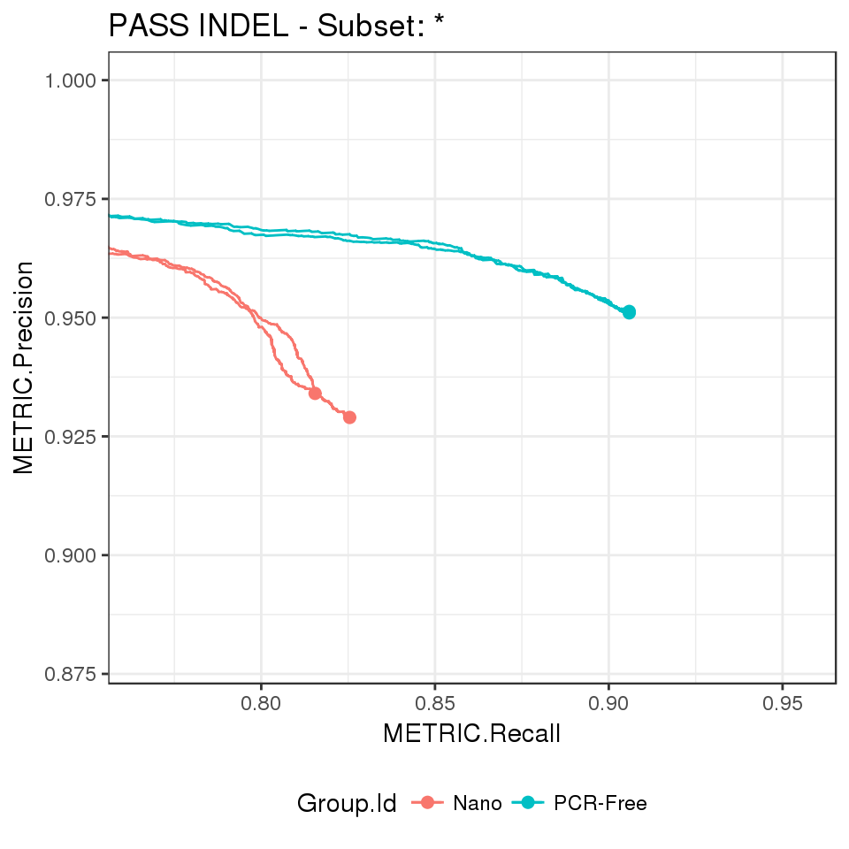

Custom metrics

# link build metrics to hap.py results
summary <- extract_metrics(happy_compare, table = "summary")
build_metrics <- extract_metrics(happy_compare, table = "build.metrics")
merged_df <- summary %>% 
  inner_join(build_metrics)

## Joining, by = c("Group.Id", "Sample.Id", "Replicate.Id", "happy_prefix", "build_metrics")

merged_df %>%
  filter(Type == "INDEL", Filter == "PASS") %>% 
  ggplot(aes(x = mean_coverage, y = METRIC.Precision, group = Group.Id)) +
  geom_point(aes(color = Group.Id)) +
  ylab("INDEL_precision")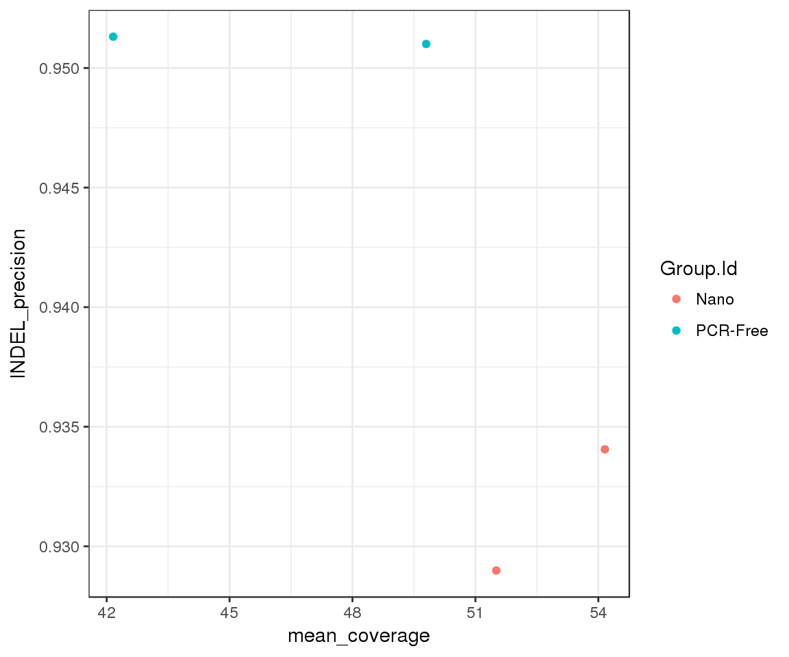

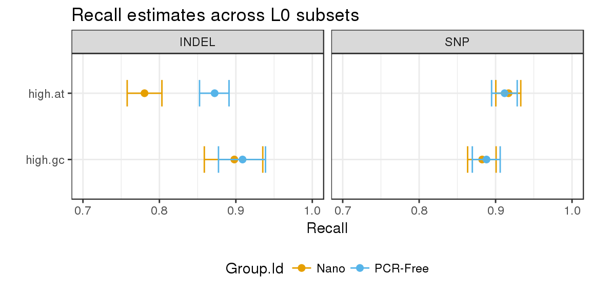
Stratified counts

# extract stratified counts and visualise highest density intervals for recall in level 0 subsets
hdi <- extract_metrics(happy_compare, table = "extended") %>% 
  filter(Subtype == "*", Filter == "PASS", Subset.Level == 0, 
         Subset %in% c("high.at", "high.gc")) %>% 
  estimate_hdi(successes_col = "TRUTH.TP", totals_col = "TRUTH.TOTAL", 
               group_cols = c("Group.Id", "Subset", "Type"), aggregate_only = FALSE)

hdi %>% 
  mutate(Subset = factor(Subset, levels = rev(unique(Subset)))) %>% 
  filter(replicate_id == ".aggregate") %>% 
  ggplot(aes(x = estimated_p, y = Subset, group = Subset)) +
    geom_point(aes(color = Group.Id), size = 2) +
    geom_errorbarh(aes(xmin = lower, xmax = upper, color = Group.Id), height = 0.4) +
    facet_grid(. ~ Type) +
    scale_colour_manual(values = c("#E69F00", "#56B4E9")) +
    theme(legend.position = "bottom") +
    ggtitle("Recall estimates across L0 subsets") +
    xlab("Recall") +
    ylab("") +
    xlim(0.7, 1)