Set up

In the present vignette we will be comparing stratified recall between a set of PCR-Free vs. Nano builds from NA12878. We will be relying on pre-processed data that we have generated by running hap.py on the VCFs from BaseSpace Data Central:

hap.py ${TRUTH_VCF} ${QUERY_VCF} -o ${OUTPUT_PREFIX} -f ${CONFIDENT_REGIONS} \
    --threads 40 --write-counts --stratification filtered_beds/stratification_config.txt --reference ${REF} \
    --roc QUAL --roc-filter LowQual --no-json

And then imported into R using the read_samplesheet() function from happyCompare:

# do not run
samplesheet_path <- "/path/to/happyCompare-master/pcrfree_vs_nano.csv"
happy_compare <- read_samplesheet(samplesheet_path, lazy = TRUE)

We will eventually end up with a happy_compare object (a list):

class(happy_compare)

## [1] "happy_compare"

sapply(happy_compare, class)

## $samplesheet
## [1] "tbl_df"     "tbl"        "data.frame"
## 
## $happy_results
## [1] "happy_result_list"
## 
## $ids
## [1] "character"

If we furhter inspect the contents of happy_results, we can see that each of its elements matches the data structures described in happyR, e.g.:

names(happy_compare$happy_results[[1]])

## [1] "summary"  "extended" "pr_curve"

Extracting data from happy_compare objects

Once we have a happy_compare object we can rely on the extract_metrics function to access our metrics of interest. Since hap.py saves stratified counts under *extended.csv files, we can use the following:

stratified_counts <- extract_metrics(happy_compare, table = "extended") %>% 
  # focus on PASS calls in level 0 subsets
  filter(Subtype == "*", Filter == "PASS", Subset.Level == 0, !grepl(pattern = "TS*", Subset)) 

This will conveniently merge hap.py results with samplesheet metadata, making downstream analysis easier:

stratified_counts

## # A tibble: 140 x 69
##    Group.Id Sample.Id   Replicate.Id
##       <chr>     <chr>          <chr>
##  1 PCR-Free   NA12878 NA12878-I30_S1
##  2 PCR-Free   NA12878 NA12878-I30_S1
##  3 PCR-Free   NA12878 NA12878-I30_S1
##  4 PCR-Free   NA12878 NA12878-I30_S1
##  5 PCR-Free   NA12878 NA12878-I30_S1
##  6 PCR-Free   NA12878 NA12878-I30_S1
##  7 PCR-Free   NA12878 NA12878-I30_S1
##  8 PCR-Free   NA12878 NA12878-I30_S1
##  9 PCR-Free   NA12878 NA12878-I30_S1
## 10 PCR-Free   NA12878 NA12878-I30_S1
## # ... with 130 more rows, and 66 more variables: happy_prefix <chr>,
## #   Type <chr>, Subtype <chr>, Subset <chr>, Filter <chr>, Genotype <chr>,
## #   QQ.Field <chr>, QQ <chr>, METRIC.Recall <dbl>, METRIC.Precision <dbl>,
## #   METRIC.Frac_NA <dbl>, METRIC.F1_Score <dbl>, FP.gt <int>, FP.al <int>,
## #   Subset.Size <dbl>, Subset.IS_CONF.Size <dbl>, Subset.Level <dbl>,
## #   TRUTH.TOTAL <int>, TRUTH.TOTAL.ti <dbl>, TRUTH.TOTAL.tv <dbl>,
## #   TRUTH.TOTAL.het <dbl>, TRUTH.TOTAL.homalt <dbl>,
## #   TRUTH.TOTAL.TiTv_ratio <dbl>, TRUTH.TOTAL.het_hom_ratio <dbl>,
## #   TRUTH.TP <int>, TRUTH.TP.ti <dbl>, TRUTH.TP.tv <dbl>,
## #   TRUTH.TP.het <dbl>, TRUTH.TP.homalt <dbl>, TRUTH.TP.TiTv_ratio <dbl>,
## #   TRUTH.TP.het_hom_ratio <dbl>, TRUTH.FN <int>, TRUTH.FN.ti <dbl>,
## #   TRUTH.FN.tv <dbl>, TRUTH.FN.het <dbl>, TRUTH.FN.homalt <dbl>,
## #   TRUTH.FN.TiTv_ratio <dbl>, TRUTH.FN.het_hom_ratio <dbl>,
## #   QUERY.TOTAL <int>, QUERY.TOTAL.ti <dbl>, QUERY.TOTAL.tv <dbl>,
## #   QUERY.TOTAL.het <dbl>, QUERY.TOTAL.homalt <dbl>,
## #   QUERY.TOTAL.TiTv_ratio <dbl>, QUERY.TOTAL.het_hom_ratio <dbl>,
## #   QUERY.TP <int>, QUERY.TP.ti <dbl>, QUERY.TP.tv <dbl>,
## #   QUERY.TP.het <dbl>, QUERY.TP.homalt <dbl>, QUERY.TP.TiTv_ratio <dbl>,
## #   QUERY.TP.het_hom_ratio <dbl>, QUERY.FP <int>, QUERY.FP.ti <dbl>,
## #   QUERY.FP.tv <dbl>, QUERY.FP.het <dbl>, QUERY.FP.homalt <dbl>,
## #   QUERY.FP.TiTv_ratio <dbl>, QUERY.FP.het_hom_ratio <dbl>,
## #   QUERY.UNK <int>, QUERY.UNK.ti <dbl>, QUERY.UNK.tv <dbl>,
## #   QUERY.UNK.het <dbl>, QUERY.UNK.homalt <dbl>,
## #   QUERY.UNK.TiTv_ratio <dbl>, QUERY.UNK.het_hom_ratio <dbl>

Downstream analysis of stratified counts

Finally, we can estimate highest density intervals to account for uncertainty in the stratified counts:

hdi <- stratified_counts %>% 
  estimate_hdi(successes_col = "TRUTH.TP", totals_col = "TRUTH.TOTAL", 
               group_cols = c("Group.Id", "Subset", "Type"), aggregate_only = FALSE)

And visualise the results using ggplot2:

hdi %>% 
  mutate(Subset = factor(Subset, rev(sort(unique(Subset))))) %>% 
  filter(replicate_id == ".aggregate") %>% 
  ggplot(aes(x = estimated_p, y = Subset, group = Subset)) +
    geom_point(aes(color = Group.Id), size = 2) +
    geom_errorbarh(aes(xmin = lower, xmax = upper, color = Group.Id), height = 0.4) +
    facet_grid(. ~ Type) +
    theme(legend.position = "bottom") +
    ggtitle("Recall estimates in L0 subsets") +
    ylab("")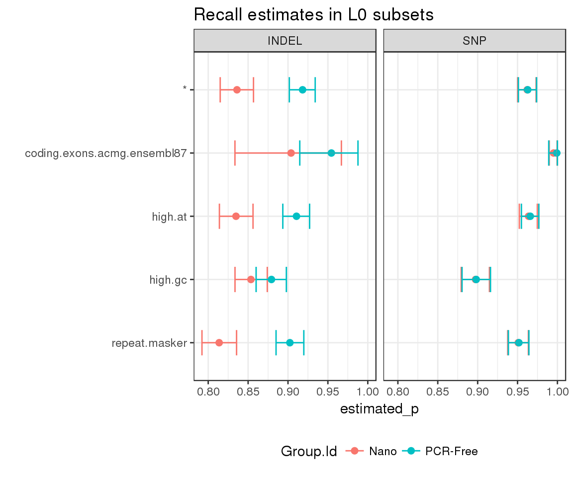

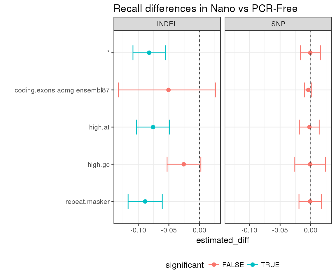
We can also evaluate the significance of the differences highlighted by our plot with compare_hdi:

hdi_diff <- compare_hdi(happy_hdi = hdi)

hdi_diff %>% 
  mutate(Subset = factor(Subset, levels = rev(sort(unique(Subset))))) %>% 
  ggplot(aes(x = estimated_diff, y = Subset, group = Subset)) +
    geom_point(aes(color = significant), size = 2) +
    geom_errorbarh(aes(xmin = lower, xmax = upper, color = significant), height = 0.4) +
    geom_vline(xintercept = 0, lty = 2, lwd = 0.25) +
    facet_grid(. ~ Type) +
    theme(legend.position = "bottom") +
    ggtitle("Recall differences in Nano vs PCR-Free") +
    ylab("")